Evaluate Stupid Back-off next-word predictions

Evaluate next-word predictions based on Stupid Back-off N-gram model on a test corpus.

eval_sbo_predictor(model, test, L = attr(model, "L"))

Arguments

model	a sbo_predictor object.
test	a character vector. Perform a single prediction on each entry of this vector (see details).
L	Maximum number of predictions for each input sentence (maximum allowed is attr(model, "L"))

Value

A tibble, containing the input $(N-1)$-grams, the true completions, the predicted completions and a column indicating whether one of the predictions were correct or not.

Details

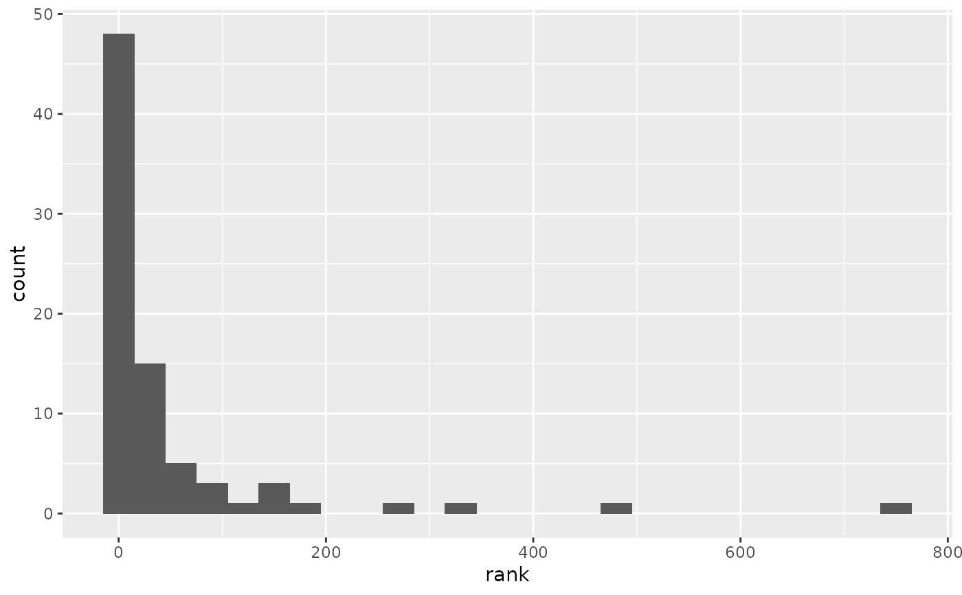
This function allows to obtain information on the quality of Stupid Back-off model predictions, such as next-word prediction accuracy, or the word-rank distribution of correct prediction, by direct test against a test set corpus. For a reasonable estimate of prediction accuracy, the different entries of the test vector should be uncorrelated documents (e.g. separate tweets, as in the twitter_test example dataset).

More in detail, eval_sbo_predictor performs the following operations:

1. Sample a single sentence from each entry of the character vector test.

2. Sample a single $N$-gram from each sentence obtained in the previous step.

3. Predict next words from the $(N-1)$-gram prefix.

4. Return all predictions, together with the true word completions.

Author

Valerio Gherardi

Examples

# \donttest{
# Evaluating next-word predictions from a Stupid Back-off N-gram model
if (suppressMessages(require(dplyr) && require(ggplot2))) {
        p <- sbo_predictor(twitter_predtable)
        set.seed(840) # Set seed for reproducibility
        test <- sample(twitter_test, 500)
        eval <- eval_sbo_predictor(p, test)
        
        ## Compute three-word accuracies
        eval %>% summarise(accuracy = sum(correct)/n()) # Overall accuracy
        eval %>% # Accuracy for in-sentence predictions
                filter(true != "<EOS>") %>%
                summarise(accuracy = sum(correct) / n())
        
        ## Make histogram of word-rank distribution for correct predictions
        dict <- attr(twitter_predtable, "dict")
        eval %>%
                filter(correct, true != "<EOS>") %>%
                transmute(rank = match(true, table = dict)) %>%
                ggplot(aes(x = rank)) + geom_histogram(binwidth = 30)
}
# }